Data visualization is key to providing effective communication of your data.
Jonathan Swan
9.1 The Data
The iris flower data set (also known as Fisher’s Iris data set) is a multivariate data set introduced by the British statistician, eugenicist, and biologist Ronald Fisher in his 1936 paper entitled, The use of multiple measurements in taxonomic problems as an example of linear discriminant analysis.
These data are part of the base R distribution and contain sepal and pedal measurements for three species if congeneric plants, Iris setosa, I. versicolor, and I. virginica.
The three species of iris in the default data set.
Here is what the data summary looks like.
summary(iris)
  Sepal.Length    Sepal.Width     Petal.Length    Petal.Width
 Min.   :4.300   Min.   :2.000   Min.   :1.000   Min.   :0.100
 1st Qu.:5.100   1st Qu.:2.800   1st Qu.:1.600   1st Qu.:0.300
 Median :5.800   Median :3.000   Median :4.350   Median :1.300
 Mean   :5.843   Mean   :3.057   Mean   :3.758   Mean   :1.199
 3rd Qu.:6.400   3rd Qu.:3.300   3rd Qu.:5.100   3rd Qu.:1.800
 Max.   :7.900   Max.   :4.400   Max.   :6.900   Max.   :2.500
       Species
 setosa    :50
 versicolor:50
 virginica :50
9.2 Basic Plotting in R
The base R comes with several built-in plotting functions, each of which is accessed through a single function with a wide array of optional arguments that modify the overall appearance.
Histograms - The Density of A Single Data Vector
hist( iris$Sepal.Length)
You can see that the default values for the hist() function label the x-axis & title on the graph have the names of the variable passed to it, with a y-axis is set to “Frequency”.
xlab & ylab: The names attached to both x- and y-axes.
main: The title on top of the graph.
breaks: This controls the way in which the original data are partitioned (e.g., the width of the bars along the x-axis).
If you pass a single number, n to this option, the data will be partitioned into n bins.
If you pass a sequence of values to this, it will use this sequence as the boundaries of bins.
col: The color of the bar (not the border)
probability: A flag as either TRUE or FALSE (the default) to have the y-axis scaled by total likelihood of each bins rather than a count of the numbrer of elements in that range.
Density - Estimating the continuous density of data
Call:
    density.default(x = iris$Sepal.Length)

Data: iris$Sepal.Length (150 obs.); Bandwidth 'bw' = 0.2736

       x               y
 Min.   :3.479   Min.   :0.0001495
 1st Qu.:4.790   1st Qu.:0.0341599
 Median :6.100   Median :0.1534105
 Mean   :6.100   Mean   :0.1905934
 3rd Qu.:7.410   3rd Qu.:0.3792237
 Max.   :8.721   Max.   :0.3968365
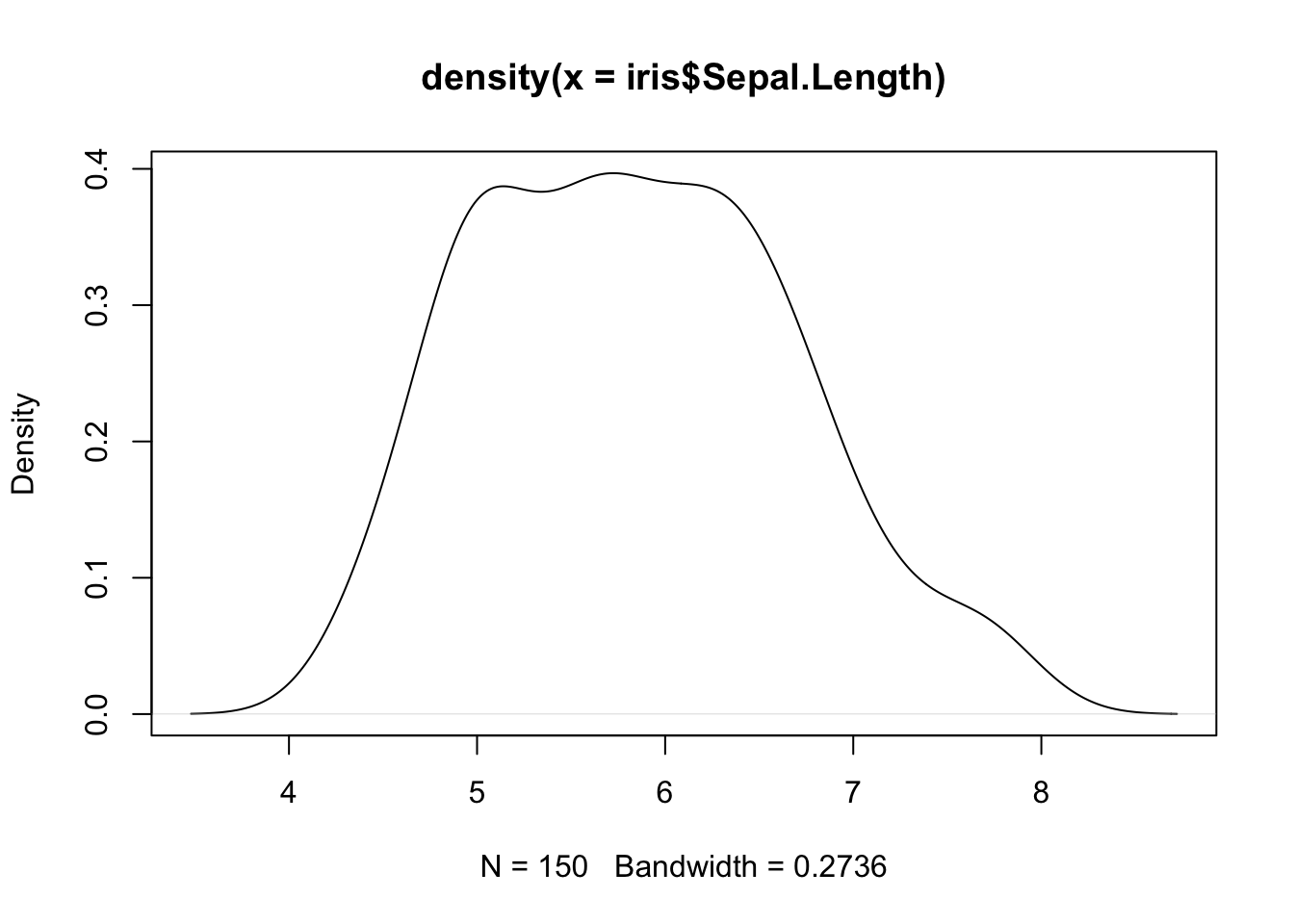
The density() function estimates a continuous probability density function for the data and returns an object that has both x and y values. In fact, it is a special kind of object.
class(d_sepal.length)
[1] "density"
Because of this, the general plot() function knows how to plot these kinds of things.
plot( d_sepal.length )
Now, the general plot() function has A TON of options and is overloaded to be able to plot all kinds of data. In addition to xlab and ylab, we modify the following:
col: Color of the line.
lwd: Line width
bty: This covers the ‘box type’, which is the square box around the plot area. I typically use bty="n" because I hate those square boxes around my plots (compare the following 2 plots to see the differences). But you do you.
xlim & ylim: These dictate the range on both the x- and y-axes. It takes a pair of values such as c(min,max) and then limits (or extends) that axis to to fill that range.
Scatter Plots - Plotting two variables
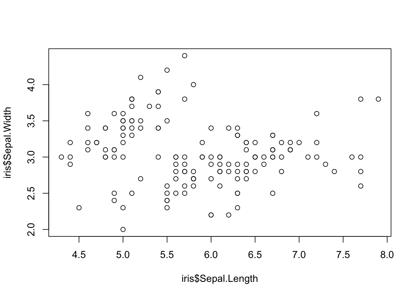
plot( iris$Sepal.Length, iris$Sepal.Width )
Here is the most general plot(). The form of the arguments to this function are x-data and then y-data. The visual representation of the data is determined by the optional values you pass (or if you do not pass any optional values, the default is the scatter plot shown above)
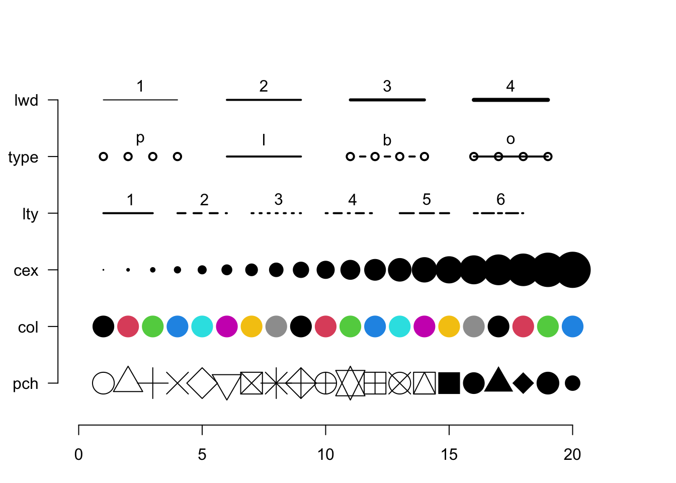
Parameter
Description
type
The kind of plot to show (’p’oint, ’l’ine, ’b’oth, or ’o’ver). A point plot is the default.
pch
The character (or symbol) being used to plot. There 26 recognized general characters to use for plotting. The default is pch=1.
col
The color of the symbols/lines that are plot.
cex
The magnification size of the character being plot. The default is cex=1 and deviation from that will increase (\(cex > 1\)) or decrease (\(0 < cex < 1\)) the scaling of the symbols.
lwd
The width of any lines in the plot.
lty
The type of line to be plot (solid, dashed, etc.)
One of the relevant things you can use the parameter pch for is to differentiate between groups of observations (such as different species for example). Instead of giving it one value, pass it a vector of values whose length is equal to that for x- and y-axis data.
Here is an example where I coerce the iris$Species data vector into numeric types and use that for symbols.
We can use the same technique to use col instead of pch. Here I make a vector of color names and then use the previously defined in the variable symbol.
raw_colors <-c("red","gold","forestgreen")colors <- raw_colors[ symbol ]colors[1:10]
In addition to the general form for the function plot(x,y) we used above, we can use an alternative designation based upon what is called the functional form. The functional form is how we designate functions in R, such as regression anlaysis. This basic syntax for this is y ~ x, that is the response variable (on the y-axis) is a function of the predictor (on the x-axis).
For simplicty, I’ll make x and y varibles pointing to the same same data as in the previous graph.
y <- iris$Sepal.Widthx <- iris$Sepal.Length
Then, the plot() function can be written as (including all the fancy additional stuff we just described):
plot( y ~ x ,
      col=colors,
      pch=20,
      bty="n",
      xlab="Sepal Length", ylab="Sepal Width")
This is much easier to read (also notice how I used serveral lines to put in all the options to the plot function for legibility).
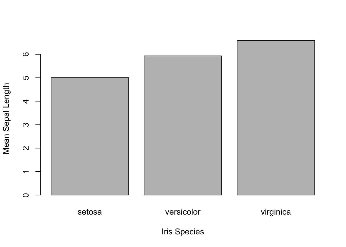
Bar Plots - Quantifying Counts
The barplot function takes a set of heights, one for each bar. Let’s quickly grab the mean length for sepals across all three species. There are many ways to do this, here are two, the first being more pedantic and the second more concise.
The iris data is in a data.frame that has a column designating the species. We can see which ones using unique().
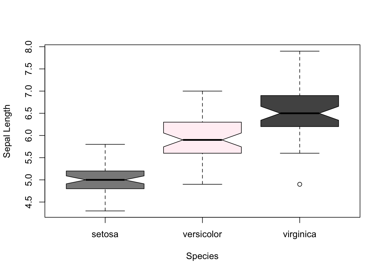
A boxplot contains a high amount of information content and is appropriate when the groupings on the x-axis are categorical. For each category, the graphical representation includes:
The median value for the raw data
A box indicating the area between the first and third quartile (e.g,. the values enclosing the 25% - 75% of the data). The top and bottoms are often referred to as the hinges of the box.
A notch (if requested), represents confidence around the estimate of the median.
Whiskers extending out to shows \(\pm 1.5 * IQR\) (the Inner Quartile Range)
Any points of the data that extend beyond the whiskers are plot as points.
For legibility, we can use the functional form for the plots as well as separate out the data.frame from the columns using the optional data= argument.
To use these colors, you can specify them by name for either all the elements
boxplot( Sepal.Length ~ Species, data = iris, col = randomColors[1],notch=TRUE, ylab="Sepal Length" )
or for each element individually.
boxplot( Sepal.Length ~ Species, data = iris, col = randomColors[1:3],notch=TRUE, ylab="Sepal Length" )
Hex Colors: You can also use hexadecimal representations of colors, which is most commonly used on the internet. A hex representation of colors consists of red, green, and blue values encoded as numbers in base 16 (e.g., the single digits 0, 1, 2, 3, 4, 5, 6, 7, 8, 9, A, B, C, D, E, F). There are a lot of great resources on the internet for color themes that report red, green, blue and hex values. I often use the coolors.co website to look for themes that go well together for slides or presentations.
Color Brewer Finally, there is an interesting website at colorbrewer2.org that has some interesting built-in palettes. There is an associated library that makes creating palettes for plots really easy and as you get more expreienced with R, you will find this very helpful. For quick visualizations and estimation of built-in color palettes, you can look at the website (below).
or look at the colors in R
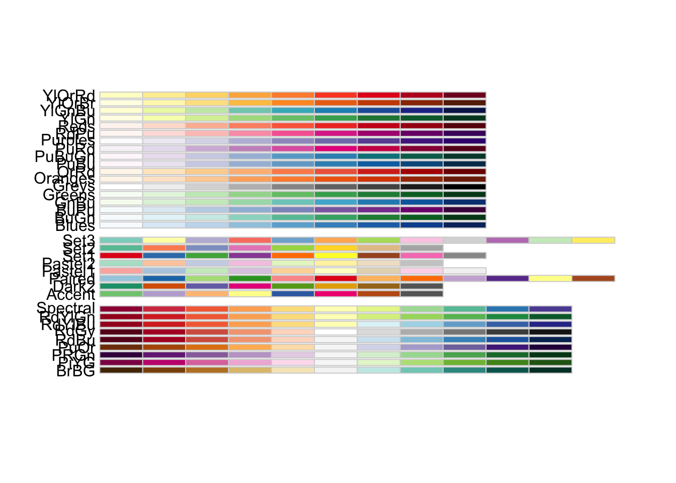
library(RColorBrewer)display.brewer.all()
There are three basic kinds of palettes: divergent, qualitative, and sequential. Each of these built-in palletes has a maximum number of colors available (though as you see below we can use them to interpolate larger sets) as well as indications if the palette is safe for colorblind individuals.
brewer.pal.info
         maxcolors category colorblind
BrBG            11      div       TRUE
PiYG            11      div       TRUE
PRGn            11      div       TRUE
PuOr            11      div       TRUE
RdBu            11      div       TRUE
RdGy            11      div      FALSE
RdYlBu          11      div       TRUE
RdYlGn          11      div      FALSE
Spectral        11      div      FALSE
Accent           8     qual      FALSE
Dark2            8     qual       TRUE
Paired          12     qual       TRUE
Pastel1          9     qual      FALSE
Pastel2          8     qual      FALSE
Set1             9     qual      FALSE
Set2             8     qual       TRUE
Set3            12     qual      FALSE
Blues            9      seq       TRUE
BuGn             9      seq       TRUE
BuPu             9      seq       TRUE
GnBu             9      seq       TRUE
Greens           9      seq       TRUE
Greys            9      seq       TRUE
Oranges          9      seq       TRUE
OrRd             9      seq       TRUE
PuBu             9      seq       TRUE
PuBuGn           9      seq       TRUE
PuRd             9      seq       TRUE
Purples          9      seq       TRUE
RdPu             9      seq       TRUE
Reds             9      seq       TRUE
YlGn             9      seq       TRUE
YlGnBu           9      seq       TRUE
YlOrBr           9      seq       TRUE
YlOrRd           9      seq       TRUE
It is very helpful to look at the different kinds of data palettes available and I’ll show you how to use them below when we color in the states based upon population size at the end of this document.
9.4 Annotations
You can easily add text onto a graph using the text() function. Here is the correlation between the sepal length and width (the function cor.test() does the statistical test).
The we can the overlay this onto an existing plot. For the text() function, we need to give the x- and y- coordinates where you want it put onto the coordinate space of the existing graph.
plot( y ~ x , col=colors, pch=20, bty="n", xlab="Sepal Length", ylab="Sepal Width")text( 7.4, 4.2, cor.text )


 or look at the colors in