Regression

Rodney Dyer, PhD

Linear Models

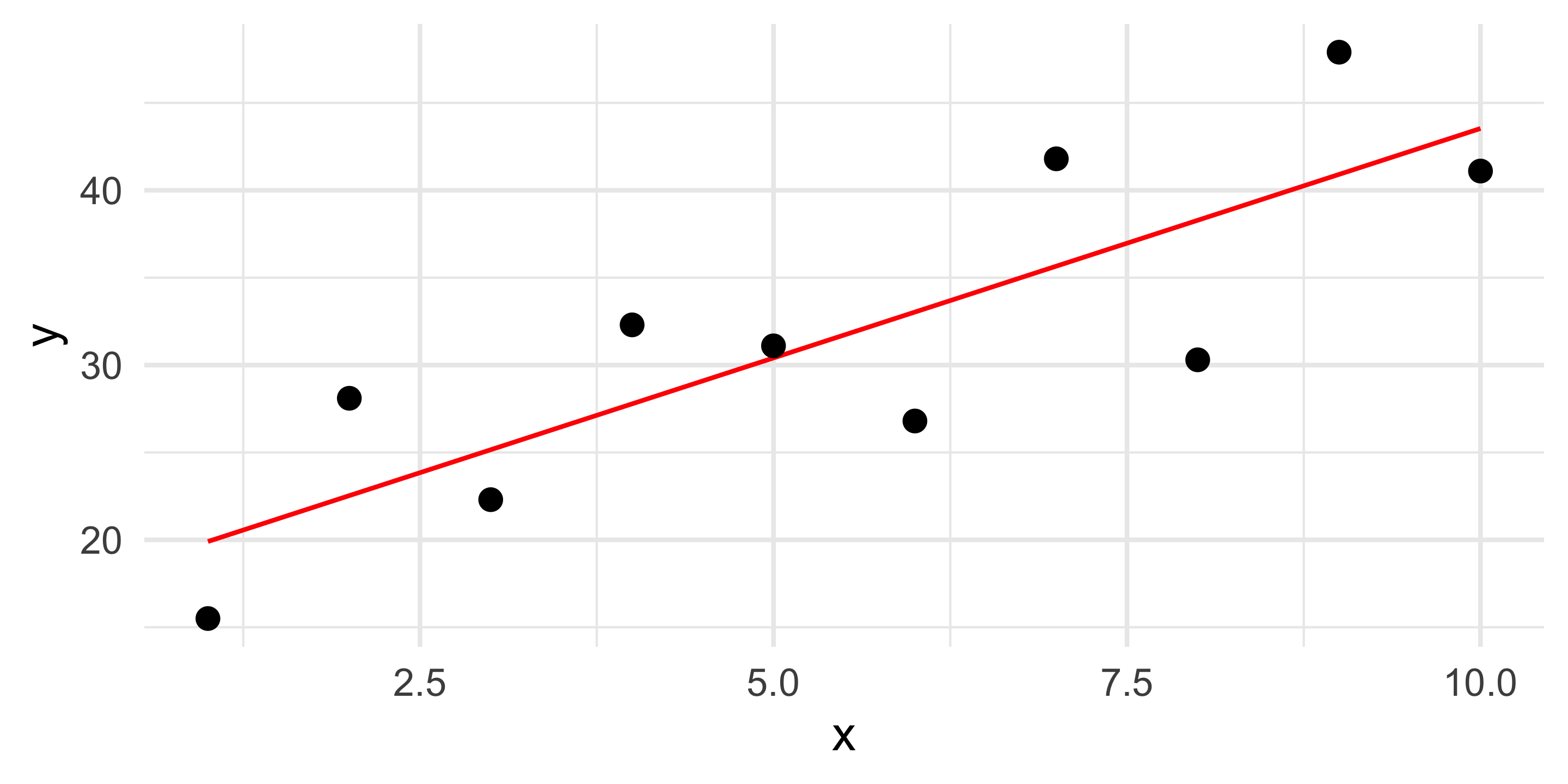
The overall goal for our introduction here, is to develop models that may be parameterized by one or more terms. The most simple model:

\[ y = \beta_0 + \beta_1 x_1 + \epsilon \]

which includes:

• An intercept ( \(\beta_0\) ),

• A slope coefficient ( \(\beta_1\) ), and

• And an error term ( \(\epsilon\) ).

Linear Models

Building Models

Random Search

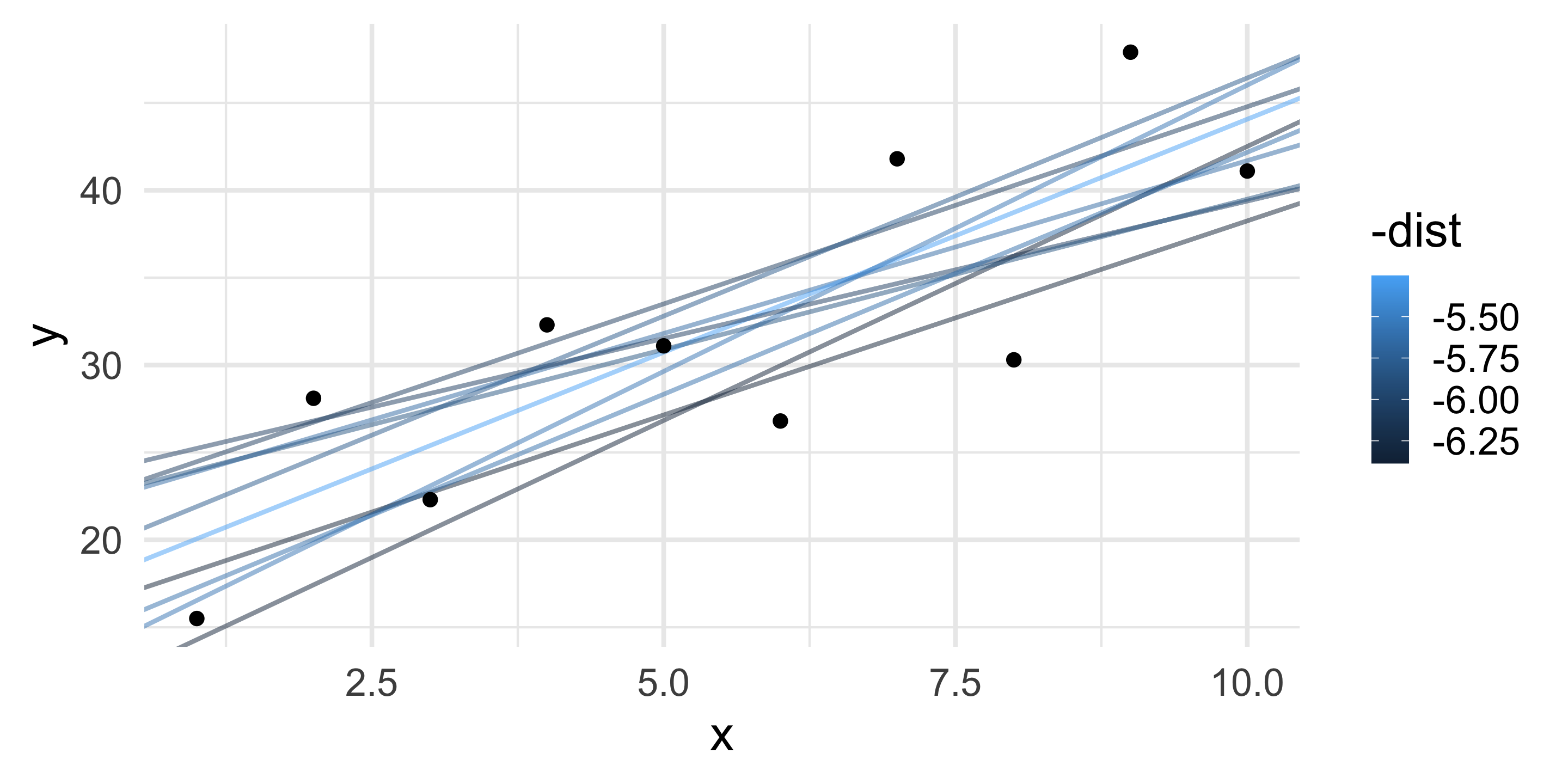
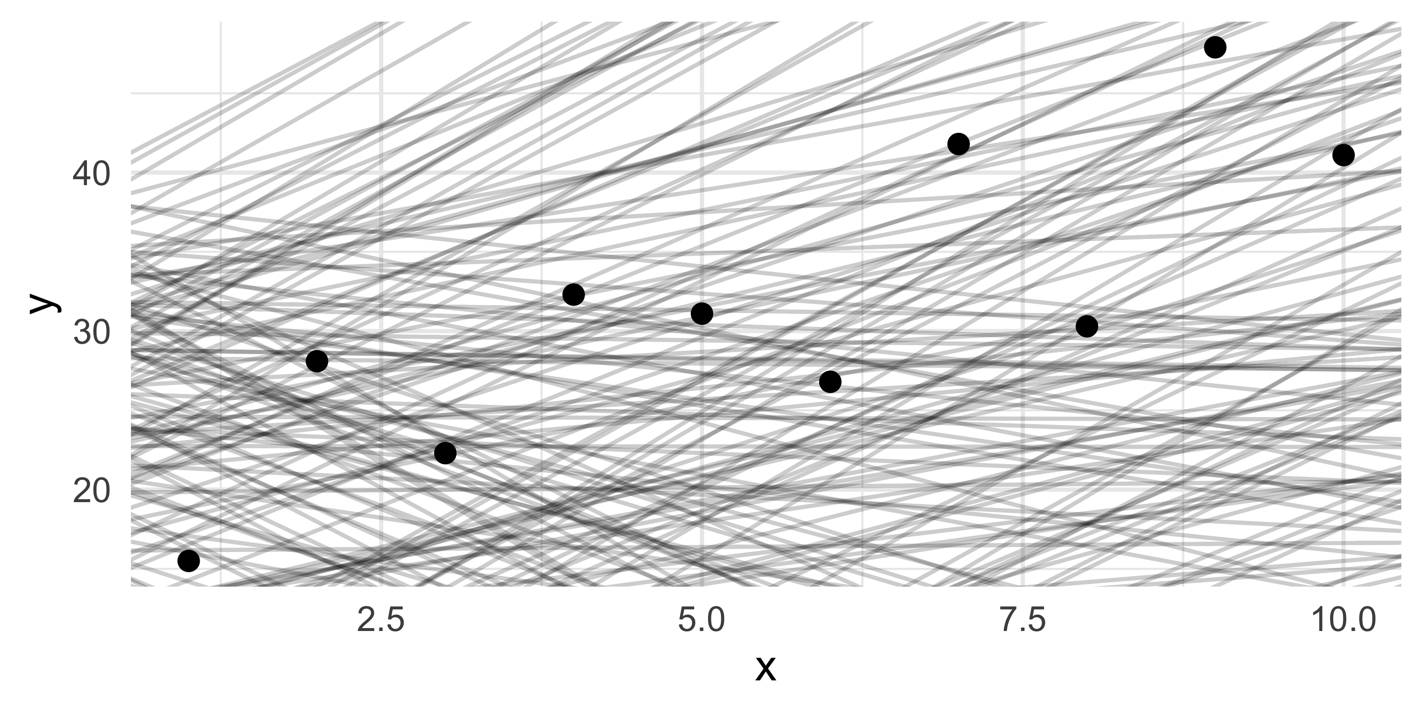
In the most fundamental form, we can make random searches

models <- data.frame( beta0 = runif(250,-20,40),
                      beta1 = runif(250, -5, 5))
summary( models )

     beta0             beta1       
 Min.   :-19.902   Min.   :-4.971  
 1st Qu.: -5.377   1st Qu.:-2.126  
 Median : 11.662   Median : 0.493  
 Mean   : 10.496   Mean   : 0.351  
 3rd Qu.: 26.400   3rd Qu.: 2.749  
 Max.   : 38.908   Max.   : 4.983  

Building A Model - Search Criterion

Searching Random Model Space

model_distance <- function( interscept, slope, X, Y ) {
  yhat <- interscept + slope * X
  diff <- Y - yhat
  return( sqrt( mean( diff ^ 2 ) ) )
}

Searching Random Model Space

models$dist <- NA
for( i in 1:nrow(models) ) {
  models$dist[i] <- model_distance( models$beta0[i],
                                    models$beta1[i],
                                    df$x,
                                    df$y )
}
head( models )

      beta0       beta1      dist
1  32.89101  4.04142654 24.320895
2  16.12870  0.05118976 17.790959
3 -14.55558 -1.31609085 54.948935
4  35.04356 -1.54833650 14.076132
5  32.08725 -1.36149237 14.467420
6  21.92174  1.97785430  5.664314

Top 10 Random Models

Take the 10 models with the smallest sum of squared distances.

ggplot()  + 
  geom_abline( aes(intercept = beta0,
                   slope = beta1, 
                   color = -dist),
               data = filter( models, 
                              rank(dist) <= 10 ),
               alpha = 0.5) + 
  geom_point( aes(x,y),
              data=df, 
              size=2) 

The Best Coefficients

ggplot( models, aes(x = beta0, y = beta1, color = -dist)) + 
  geom_point( data = filter( models, rank(dist) <= 10), 
              color = "red",  size = 4) + 
  geom_point()

Systematic Grid Search

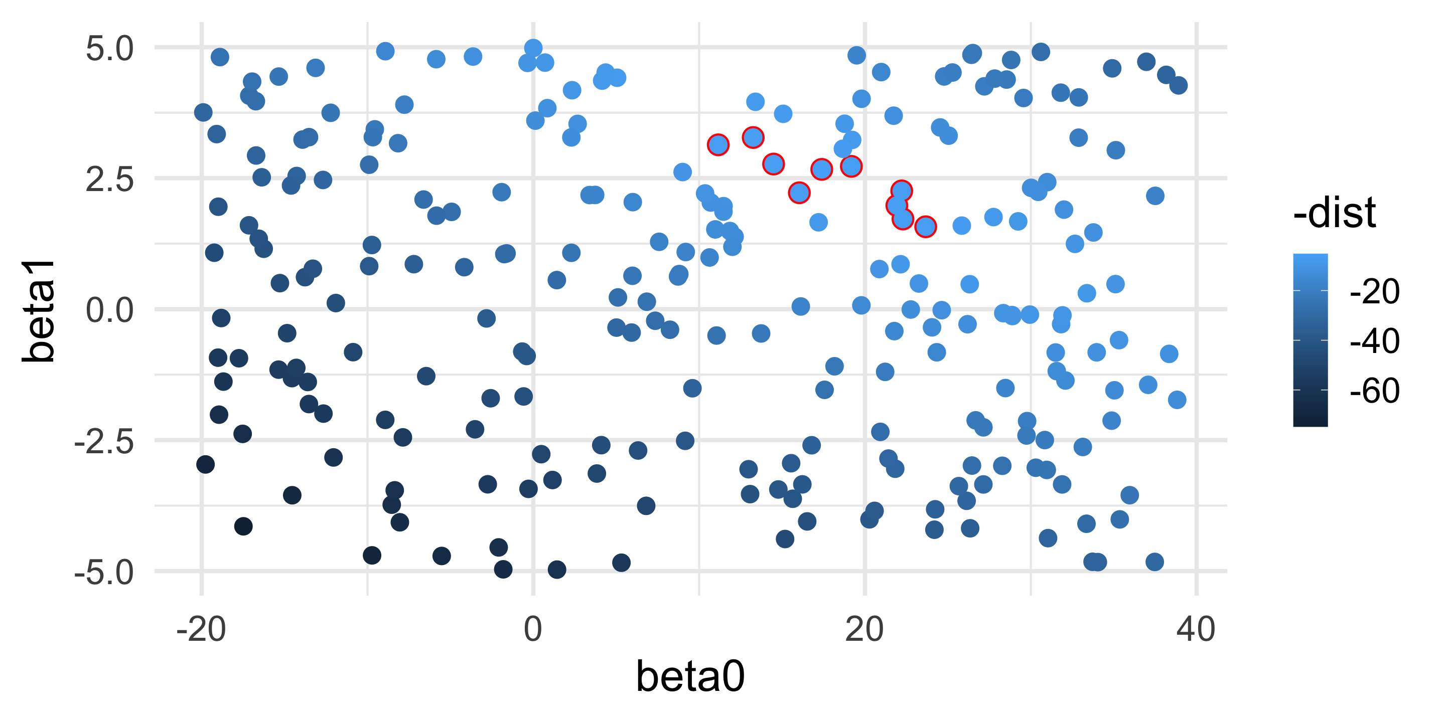
We could then systematically search the \(\beta_0\), \(\beta_1\) response space for the best set of coefficients.

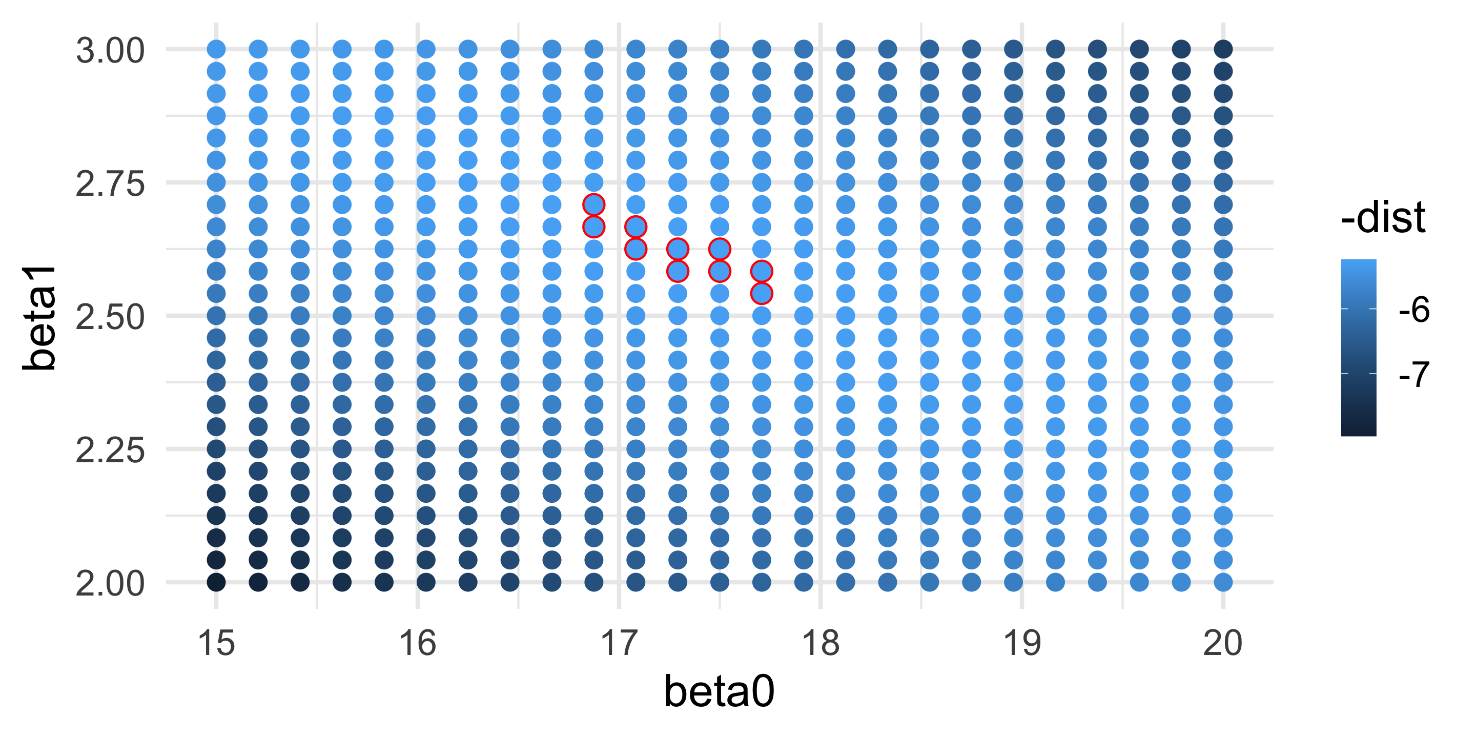
grid <- expand.grid( beta0 = seq(15, 
                                 20, 
                                 length = 25),
                     beta1 = seq(2, 
                                 3, 
                                 length = 25))
grid$dist <- NA
for( i in 1:nrow(grid) ) {
  grid$dist[i] <- model_distance( grid$beta0[i],
                                  grid$beta1[i],
                                  df$x,
                                  df$y )
}

ggplot( grid, aes(x = beta0, 
                  y = beta1,
                  color = -dist)) + 
  geom_point( data = filter( grid, 
                             rank(dist) <= 10), 
              color = "red",
              size = 4) +
  geom_point()

Our Friend Least Squares Regression

 

Specifying a Formula

For R to perform these analyses for us, we need to be able to specify the function that we will use to represent the data (just like we did for plot(y~x)). Assuming the predictor is named x and the response is y, we have:

Single Predictor Model

y ~ x

Multiple Additive Predictors

y ~ x1 + x2 

Interaction Terms

y ~ x1 + x2 + x1*x2

Fitting A Model

The easiest model.

fit <- lm( y ~ x, data = df )
fit 

Call:
lm(formula = y ~ x, data = df)

Coefficients:
(Intercept)            x  
     17.280        2.625  

Model Summaries

Summaries of the overal model components.

summary( fit )

Call:
lm(formula = y ~ x, data = df)

Residuals:
    Min      1Q  Median      3Q     Max 
-7.9836 -4.0182 -0.8709  5.3064  6.9909 

Coefficients:
            Estimate Std. Error t value Pr(>|t|)   
(Intercept)   17.280      4.002   4.318  0.00255 **
x              2.626      0.645   4.070  0.00358 **
---
Signif. codes:  0 '***' 0.001 '**' 0.01 '*' 0.05 '.' 0.1 ' ' 1

Residual standard error: 5.859 on 8 degrees of freedom
Multiple R-squared:  0.6744,    Adjusted R-squared:  0.6337 
F-statistic: 16.57 on 1 and 8 DF,  p-value: 0.003581

Components within the Summary Object

Like cor.test(), the object returned from lm() and its summary object have several internal components that you may use.

names( fit )

 [1] "coefficients"  "residuals"     "effects"       "rank"         
 [5] "fitted.values" "assign"        "qr"            "df.residual"  
 [9] "xlevels"       "call"          "terms"         "model"        

 

names( summary( fit ) )

 [1] "call"          "terms"         "residuals"     "coefficients" 
 [5] "aliased"       "sigma"         "df"            "r.squared"    
 [9] "adj.r.squared" "fstatistic"    "cov.unscaled" 

Components within the Summary Object

The probability can be found by looking at the data in the F-Statistic and then asking the F-distribution for the probability associated with the value of the test statistic and the degrees of freedom for both the model and the residuals.

summary( fit )$fstatistic 

   value    numdf    dendf 
16.56838  1.00000  8.00000 

The Summary Object

When you print out the summary( fit ) object, it uses the fstatistic to estimate a P-value. If we need that P-value directly, this is how it is done.

get_pval <- function( model ) {
  f <- summary( model )$fstatistic[1]
  df1 <- summary( model )$fstatistic[2]
  df2 <- summary( model )$fstatistic[3]
  p <- as.numeric( 1.0 - pf( f, df1, df2 ) )
  return( p  )
}

get_pval( fit )

[1] 0.0035813

So You Have a Model, Now What?

Model Diagnostics - Residuals

plot( fit, which = 1 )

Normality Of the Data

plot( fit, which = 2 )

Leverage

plot( fit, which=5 )

Decomposition of Variance

The terms in this table are:

• Degrees of Freedom (df): representing 1 degree of freedom for the model, and N-1 for the residuals.

Decomposition of Variance

The terms in this table are:

• Sums of Squared Deviations:
  • \(SS_{Total} = \sum_{i=1}^N (y_i - \bar{y})^2\)
  • \(SS_{Model} = \sum_{i=1}^N (\hat{y}_i - \bar{y})^2\), and
  • \(SS_{Residual} = SS_{Total} - SS_{Model}\)

Decomposition of Variance

The terms in this table are:

• Mean Squares (Standardization of the Sums of Squares for the degrees of freedom)
  • \(MS_{Model} = \frac{SS_{Model}}{df_{Model}}\)
  • \(MS_{Residual} = \frac{SS_{Residual}}{df_{Residual}}\)

Decomposition of Variance

The terms in this table are:

• The \(F\)-statistic is from a known distribution and is defined by the ratio of Mean Squared values.

• Pr(>F) is the probability associated the value of the \(F\)-statistic and is dependent upon the degrees of freedom for the model and residuals.

Decomposition of Variance

The classis ANOVA Table

anova( fit )

Analysis of Variance Table

Response: y
          Df Sum Sq Mean Sq F value   Pr(>F)   
x          1 568.67  568.67  16.568 0.003581 **
Residuals  8 274.58   34.32                    
---
Signif. codes:  0 '***' 0.001 '**' 0.01 '*' 0.05 '.' 0.1 ' ' 1

Variance Exaplained

summary( fit )

Call:
lm(formula = y ~ x, data = df)

Residuals:
    Min      1Q  Median      3Q     Max 
-7.9836 -4.0182 -0.8709  5.3064  6.9909 

Coefficients:
            Estimate Std. Error t value Pr(>|t|)   
(Intercept)   17.280      4.002   4.318  0.00255 **
x              2.626      0.645   4.070  0.00358 **
---
Signif. codes:  0 '***' 0.001 '**' 0.01 '*' 0.05 '.' 0.1 ' ' 1

Residual standard error: 5.859 on 8 degrees of freedom
Multiple R-squared:  0.6744,    Adjusted R-squared:  0.6337 
F-statistic: 16.57 on 1 and 8 DF,  p-value: 0.003581

Relationship Between \(R^2\) & \(r\)

How much of the variation is explained?

\[ R^2 = \frac{SS_{Model}}{SS_{Total}} \]

c( `Regression R^2` = summary( fit )$r.squared,
   `Squared Correlation` = as.numeric( cor.test( df$x, df$y )$estimate^2 ) )

     Regression R^2 Squared Correlation 
          0.6743782           0.6743782 

The square of the Pearson Correlation is equal to R

Helper Functions

Grabbing the predicted values \(\hat{y}\) from the model.

df$yhat <- predict( fit )
df %>% 
  ggplot( aes(x,yhat) ) + geom_line() + geom_point() +
  geom_point( aes(y=y), col="darkred", size=2)

Helper Functions - Residuals

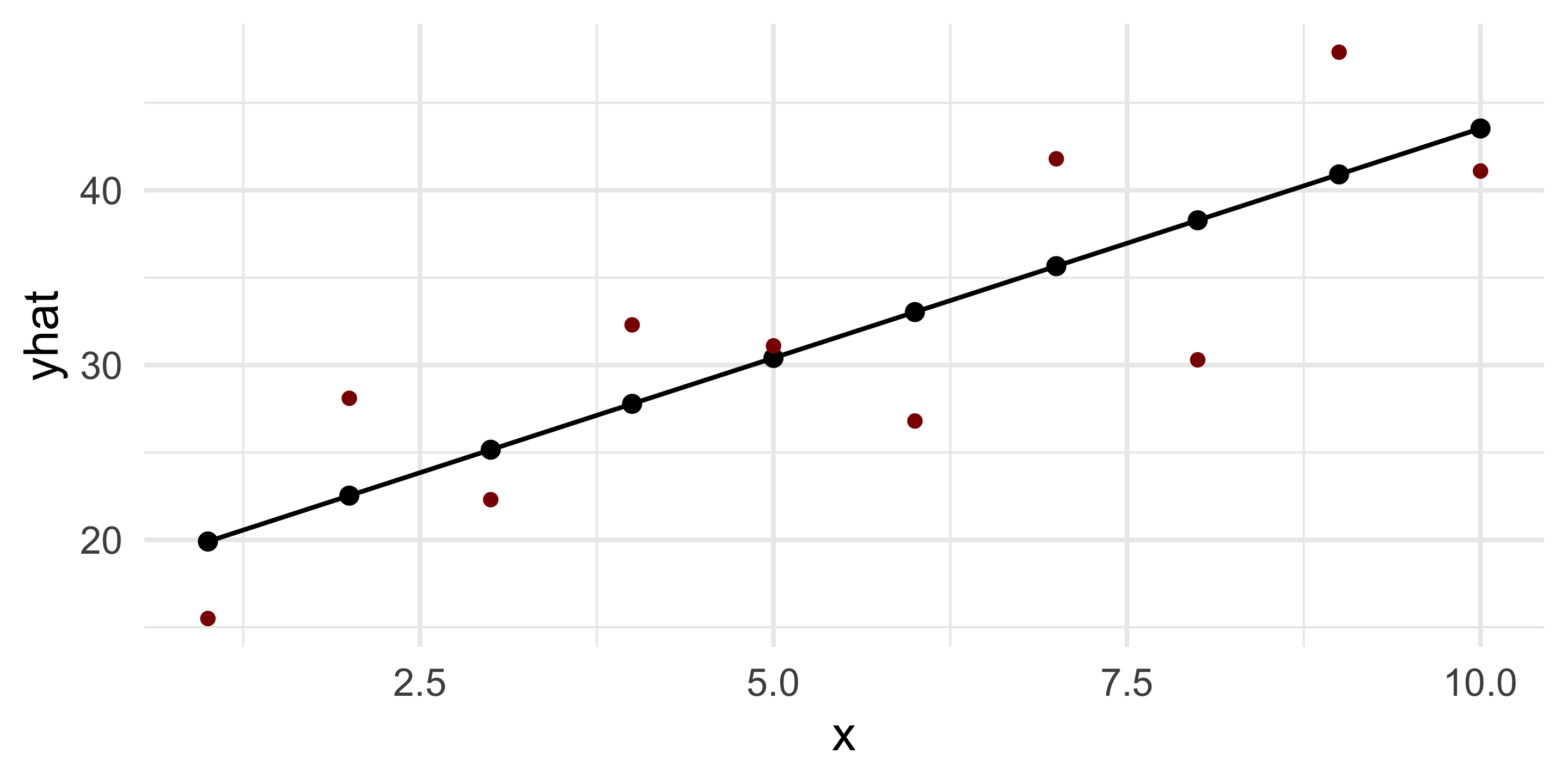
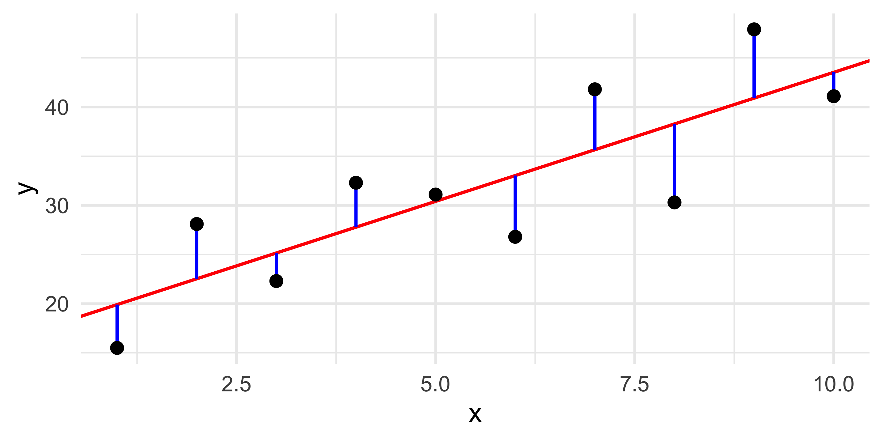
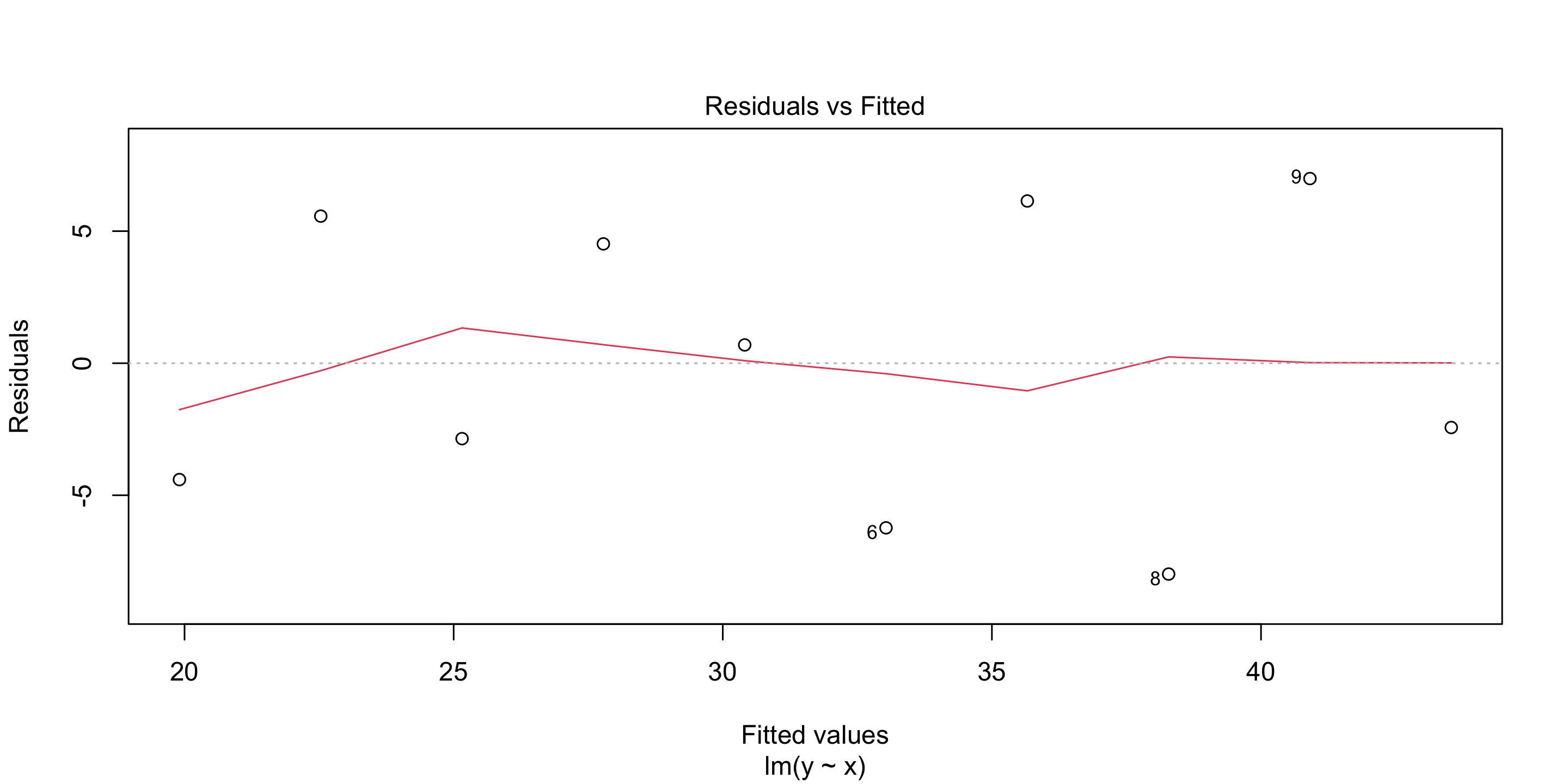
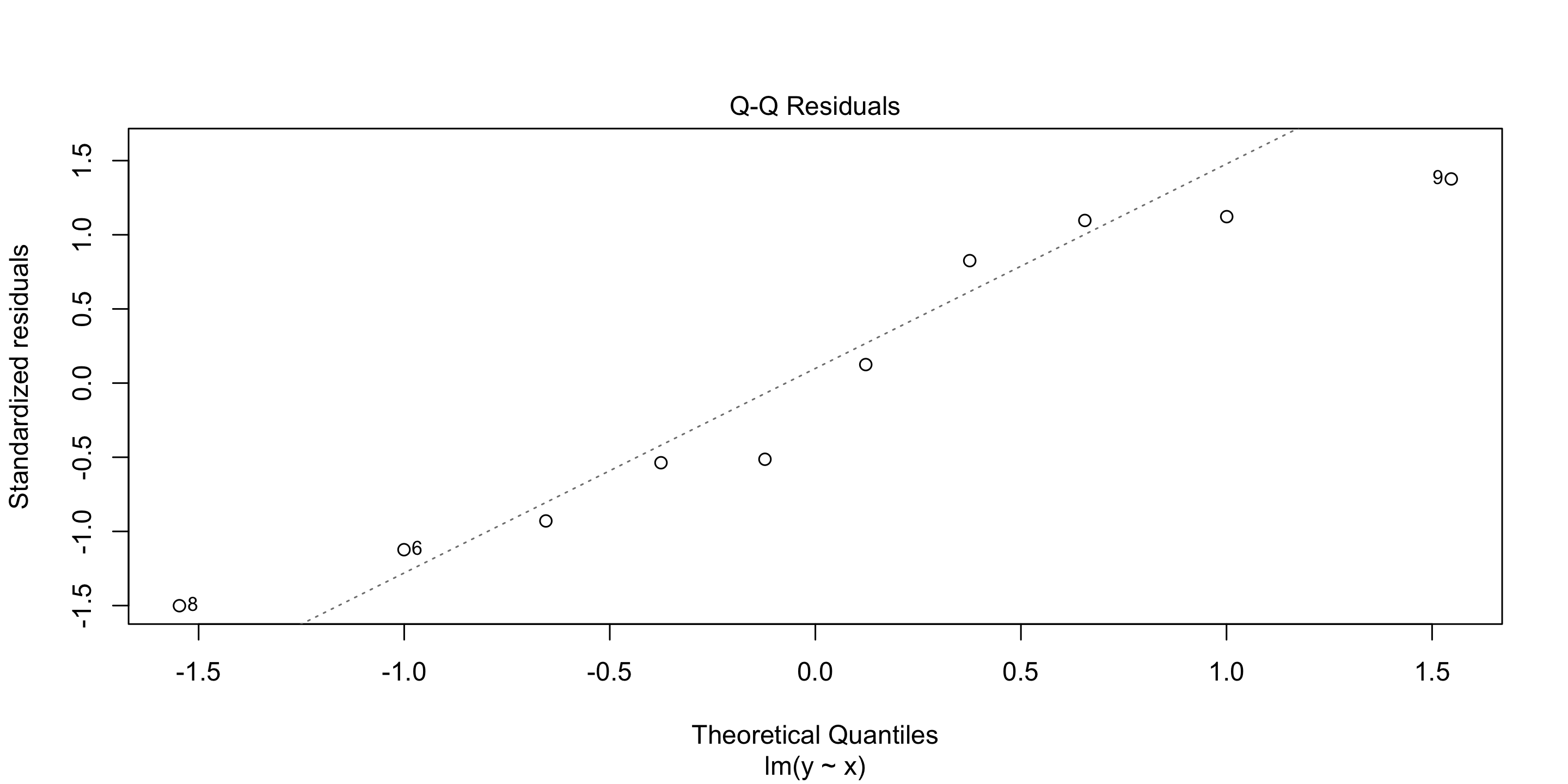
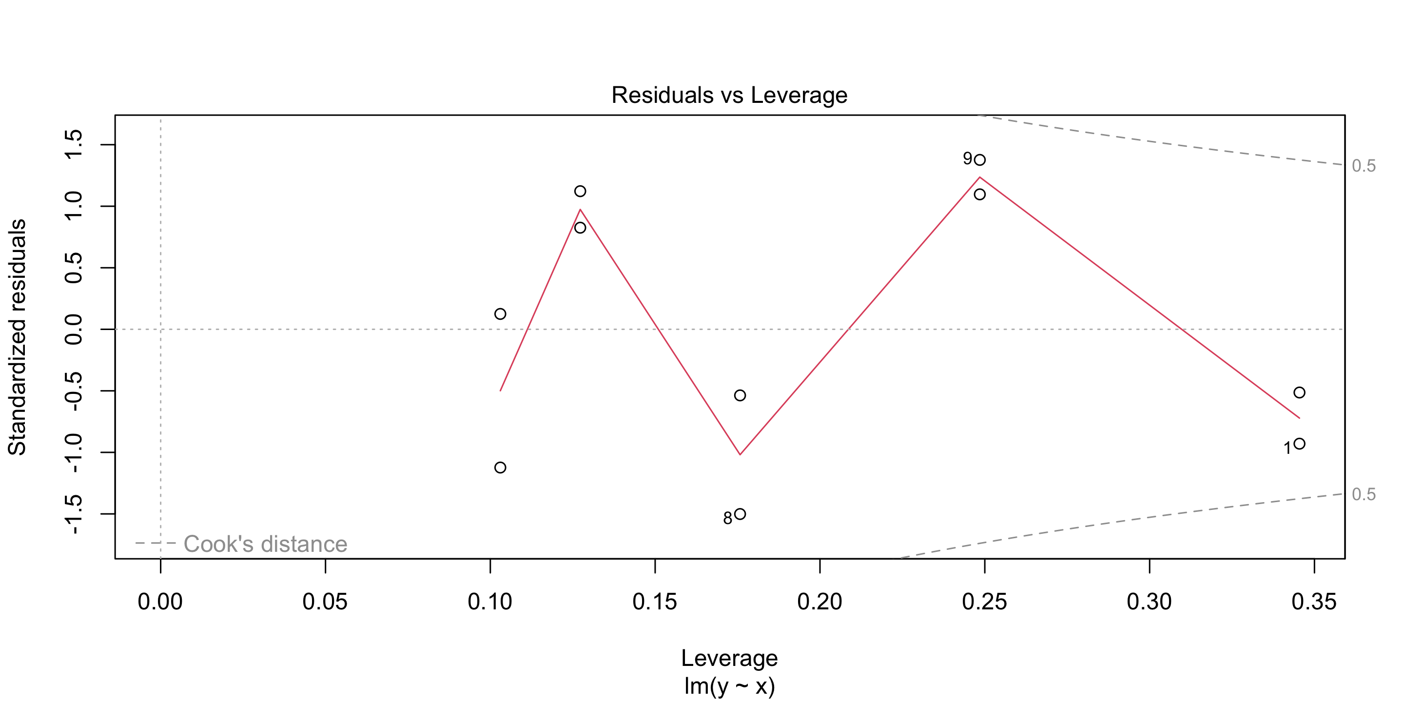
The residuals are the distances between the observed value and its corresponding value on the fitted line.

df$residuals <- residuals( fit ) 
df %>%
  ggplot( aes(yhat, residuals) ) + 
  geom_point() + 
  geom_abline( slope=0,intercept=0, color="red")

Comparing Models

What Makes One Model Better

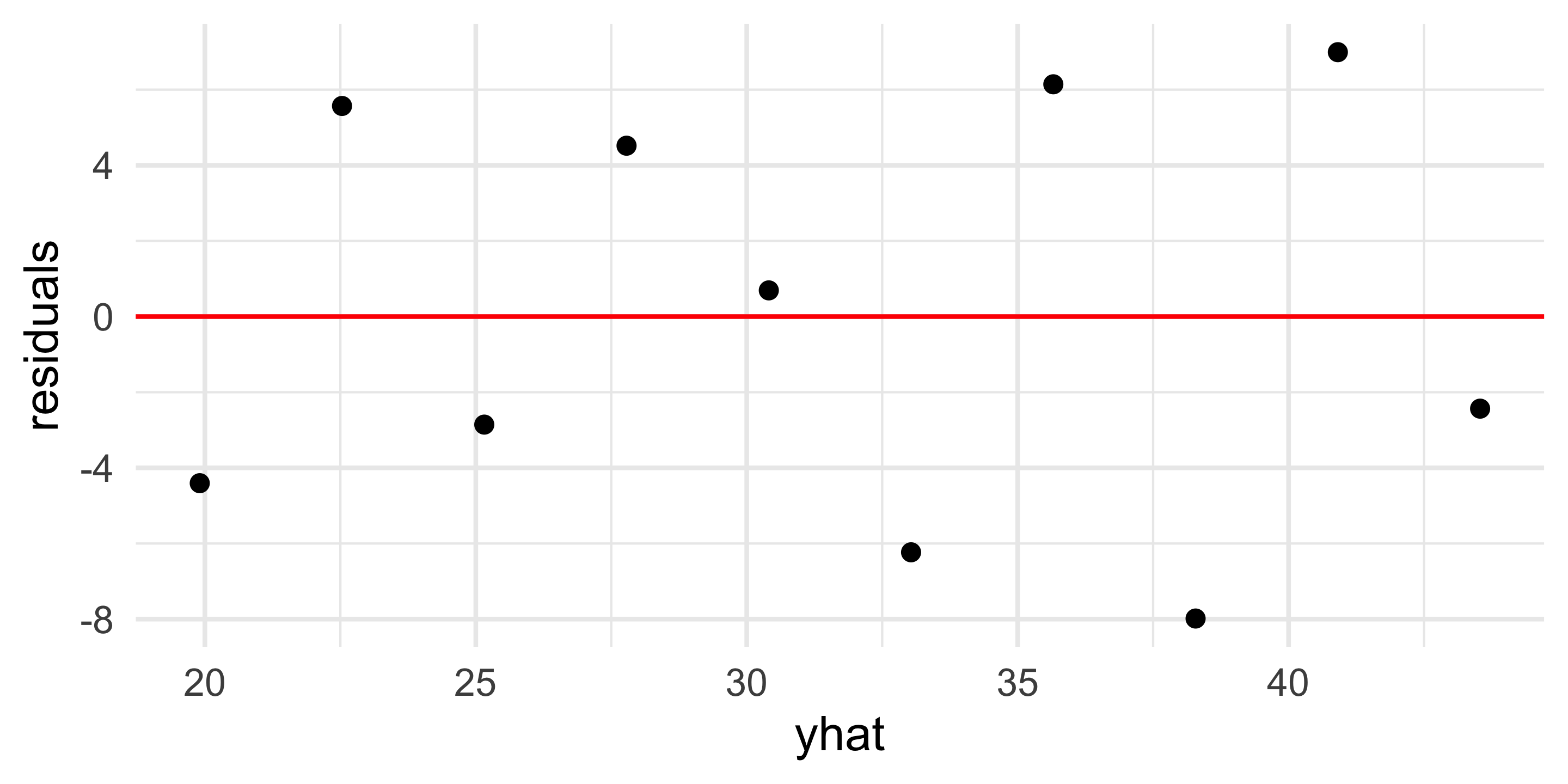
There are two parameters that we have already looked at that may help. These are:

• The \(P-value\): Models with smaller probabilities could be considered more informative.

• The \(R^2\): Models that explain more of the variation may be considered more informative.

New Data Set

Let’s start by looking at some air quality data, that is built into R as an example data set.

airquality %>%
  select( -Month, -Day ) -> df.air
summary( df.air )

     Ozone           Solar.R           Wind             Temp      
 Min.   :  1.00   Min.   :  7.0   Min.   : 1.700   Min.   :56.00  
 1st Qu.: 18.00   1st Qu.:115.8   1st Qu.: 7.400   1st Qu.:72.00  
 Median : 31.50   Median :205.0   Median : 9.700   Median :79.00  
 Mean   : 42.13   Mean   :185.9   Mean   : 9.958   Mean   :77.88  
 3rd Qu.: 63.25   3rd Qu.:258.8   3rd Qu.:11.500   3rd Qu.:85.00  
 Max.   :168.00   Max.   :334.0   Max.   :20.700   Max.   :97.00  
 NA's   :37       NA's   :7                                       

Base Models - What Influences Ozone

Individually, we can estimate a set of first-order models.

\[ y = \beta_0 + \beta_1 x_1 + \epsilon \]

fit.solar <- lm( Ozone ~ Solar.R, data = df.air )
fit.temp <- lm( Ozone ~ Temp, data = df.air )
fit.wind <- lm( Ozone ~ Wind, data = df.air )

Base Models - What Influences Ozone

Model parameters predicting mean ozone in parts per billion mearsured in New York during the period of 1 May 1973 - 30 September 1973 as predicted by Temperature, Windspeed, and Solar Radiation.

Model	R2	P
Ozone ~ Solar	0.121	1.79e-04
Ozone ~ Temp	0.488	0.00e+00
Ozone ~ Wind	0.362	9.27e-13

More Complicated Models

Multiple Regression Model - Including more than one predictors.

\(y = \beta_0 + \beta_1 x_1 + \beta_2 x_2 + \epsilon\)

fit.temp.wind <- lm( Ozone ~ Temp + Wind, data = df.air )
fit.temp.solar <- lm( Ozone ~ Temp + Solar.R, data = df.air )
fit.wind.solar <- lm( Ozone ~ Wind + Solar.R, data = df.air )

More Complicated Models

Model parameters predicting mean ozone in parts per billion mresured in New York during the period of 1 May 1973 - 30 September 1973.

Model	R2	P
Ozone ~ Solar	0.121	1.79e-04
Ozone ~ Temp	0.488	0.00e+00
Ozone ~ Wind	0.362	9.27e-13
Ozone ~ Temp + Wind	0.569	0.00e+00
Ozone ~ Temp + Solar	0.510	0.00e+00
Ozone ~ Wind + Solar	0.449	9.99e-15

For Completeness

How about all the predictors. \(y = \beta_0 + \beta_1 x_1 + \beta_2 x_2 + \beta_3 x_3 + \epsilon\)

fit.all <- lm( Ozone ~ Solar.R + Temp + Wind, data = df.air )

For Completeness

Model	R2	P
Ozone ~ Solar	0.1213419	1.79e-04
Ozone ~ Temp	0.4877072	0.00e+00
Ozone ~ Wind	0.3618582	9.27e-13
Ozone ~ Temp + Wind	0.5687097	0.00e+00
Ozone ~ Temp + Solar	0.5103167	0.00e+00
Ozone ~ Wind + Solar	0.4494936	9.99e-15
Ozone ~ Temp + Wind + Solar	0.6058946	0.00e+00

\(R^2\) Inflation

Any variable added to a model will be able to generate Sums of Squares (even if it is a small amount). So, adding variables may artifically inflate the Model Sums of Squares.

Example:

What happens if I add just random data to the regression models? How does \(R^2\) change?

Random Data Effects

Original data in models.

Models	R2
Ozone ~ Temp	0.4877
Ozone ~ Wind	0.3619
Ozone ~ Solar	0.1213
Ozone ~ Temp + Wind	0.5687
Ozone ~ Temp + Solar	0.5103
Ozone ~ Wind + Solar	0.4495
Ozone ~ Temp + Wind + Solar	0.6059

Random Data Effects

Original full model + X random variables

Models	R2
Ozone ~ Temp + Wind + Solar + 1 Random Variables	0.6061
Ozone ~ Temp + Wind + Solar + 2 Random Variables	0.6065
Ozone ~ Temp + Wind + Solar + 3 Random Variables	0.6067
Ozone ~ Temp + Wind + Solar + 4 Random Variables	0.6134
Ozone ~ Temp + Wind + Solar + 5 Random Variables	0.6134
Ozone ~ Temp + Wind + Solar + 6 Random Variables	0.6164
Ozone ~ Temp + Wind + Solar + 7 Random Variables	0.6170
Ozone ~ Temp + Wind + Solar + 8 Random Variables	0.6186

Perfect - My Models RULE

I can just add random variables to my model and always get an awesome fit!

 

 

Not so fast Bevis!

Model Comparisons

Akaike Information Criterion (AIC) is a measurement that allows us to compare models while penalizing for adding new parameters.

\(AIC = -2 \ln L + 2p\)

The criterion here are to find models with the lowest AIC values.

Comparisons

To compare, we evaluate the differences in AIC for alternative models.

\(\delta AIC = AIC - min( AIC )\)

AIC & ∂AIC

Models	R2	AIC	deltaAIC
Ozone ~ Temp	0.488	1067.706	68.989
Ozone ~ Wind	0.362	1093.187	94.470
Ozone ~ Solar	0.121	1083.714	84.997
Ozone ~ Temp + Wind	0.569	1049.741	51.024
Ozone ~ Temp + Solar	0.510	1020.820	22.103
Ozone ~ Wind + Solar	0.449	1033.816	35.098
Ozone ~ Temp + Wind + Solar	0.606	998.717	0.000
Ozone ~ Temp + Wind + Solar + 1 Random Variables	0.606	1000.653	1.936
Ozone ~ Temp + Wind + Solar + 2 Random Variables	0.607	1002.545	3.828
Ozone ~ Temp + Wind + Solar + 3 Random Variables	0.607	1004.498	5.781
Ozone ~ Temp + Wind + Solar + 4 Random Variables	0.613	1004.592	5.875
Ozone ~ Temp + Wind + Solar + 5 Random Variables	0.613	1006.592	7.874
Ozone ~ Temp + Wind + Solar + 6 Random Variables	0.616	1007.727	9.010
Ozone ~ Temp + Wind + Solar + 7 Random Variables	0.617	1009.542	10.825
Ozone ~ Temp + Wind + Solar + 8 Random Variables	0.619	1011.070	12.353

Questions

If you have any questions, please feel free to either post them as an “Issue” on your copy of this GitHub Repository, post to the Canvas discussion board for the class, or drop me an email.