# A tibble: 6 × 3
   Year `Nicolas Cage Movies` `Drowning Deaths in Pools`
  <int>                 <dbl>                      <dbl>
1  1999                     2                        109
2  2000                     2                        102
3  2001                     2                        102
4  2002                     3                         98
5  2003                     1                         85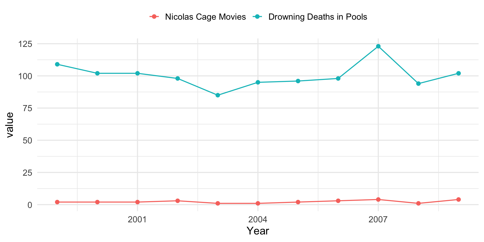
6 2004 1 95Models of Correlation
Coincident change in pairs of variables
Beer Judge Certification Program
Recognized Beer Styles
100 Distinct Styles (not just IPA’s & that yellow American Corn Lager!)
Global & Regional Styles
Quantitative Characteristics
- IBU, SRM, ABV, OG, FG
Qualitative Characteristics
- Overall Impression, Aroma, Appearance, Flavor, & Mouthfeel

The BJCP Style Guidelines exist for beer, mead, and ciders.
Basic Yeast Types

Not including sour beers, which use yeast and bacteria mixtures.
Dissolved Sugars - OG & FG
The more sugar in the wort, the more food for the yeast to work on, and the more alcohol that may be produced.
The difference between the gravities before and after fermentation can be used to estimate ABV.

Bitterness
Bitterness is created by the addition of herbs.

Color
The color of the beer is quantified using the Standard Reference Method (SRM) scale.

Field Trip!
Normality
In general, data we work with is assumed to follow a Normal distribution with parameters \(\mu\) and \(\sigma\), often denoted as \(N(\mu,\sigma)\), which can be parameterized as:
\[ f(x) = \frac{1}{\sigma\sqrt{2\pi}}e^{-\frac{1}{2}(\frac{x - \mu}{\sigma})} \]
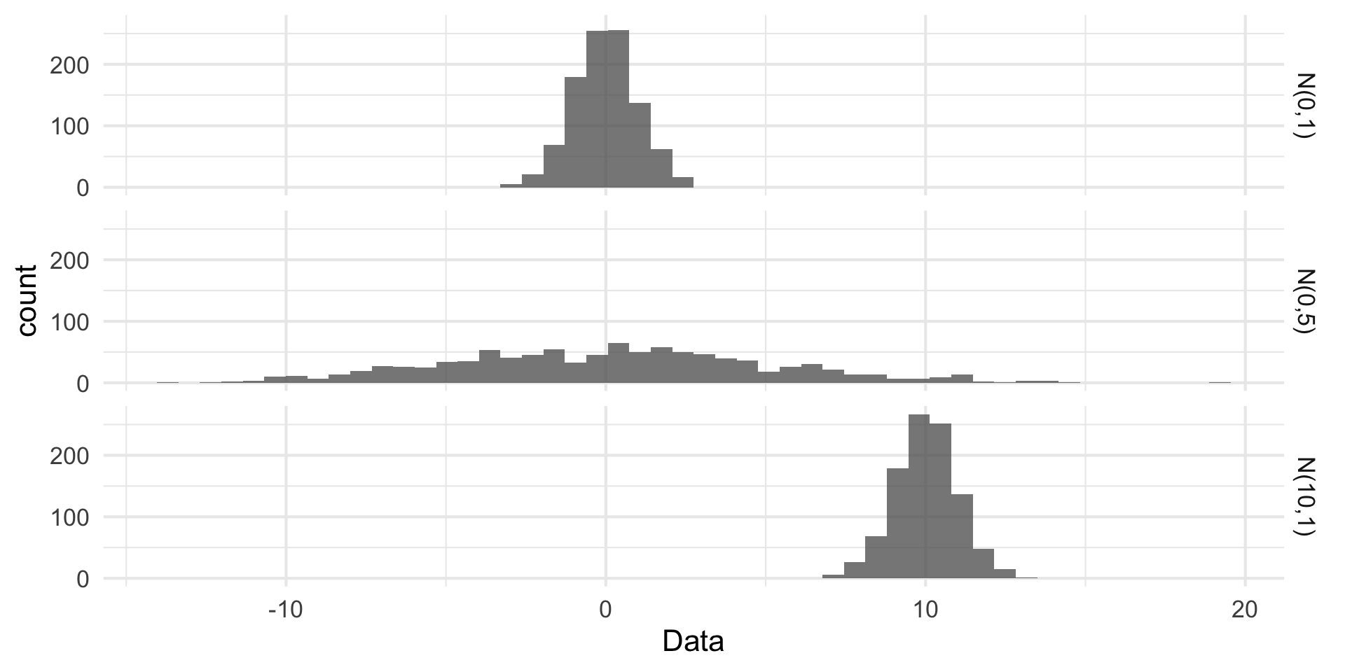
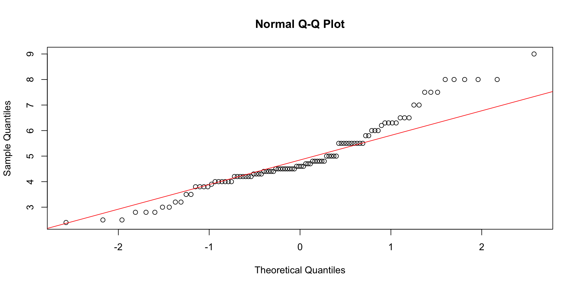
Visualizing Normality
Visualizing the ‘normality’ of the data using built-in functions.
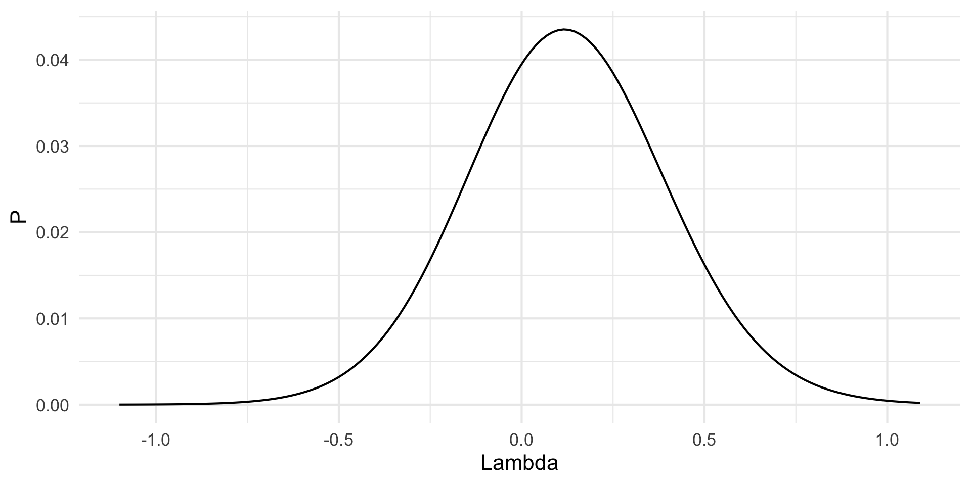
Data Transformations - Box Cox
Equality of Variance
It is assumed that the variance of the data are
Independence of Data
The samples you collect, and the way that you design your experiments are most important to ensure that your data are individually independent. You need to think about this very carefully as you design your experiments.

Visual Examples

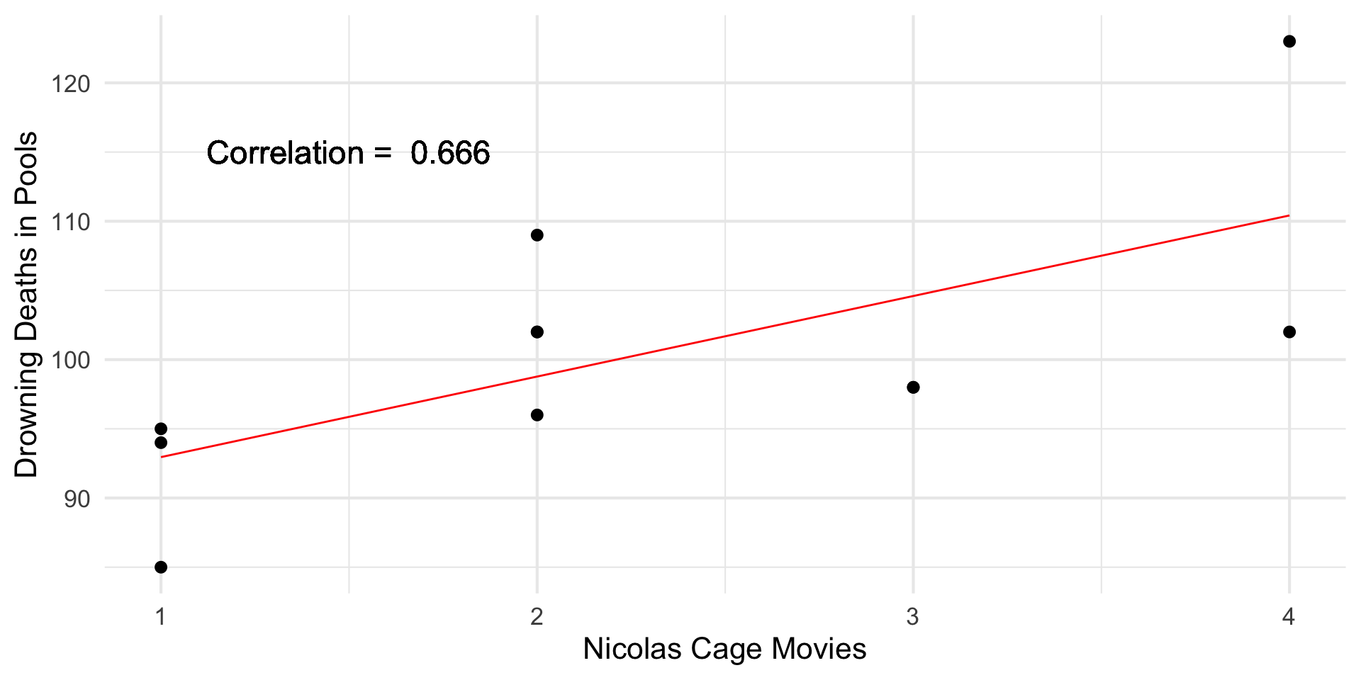
Figure 1: Data and associated correlation statistics.
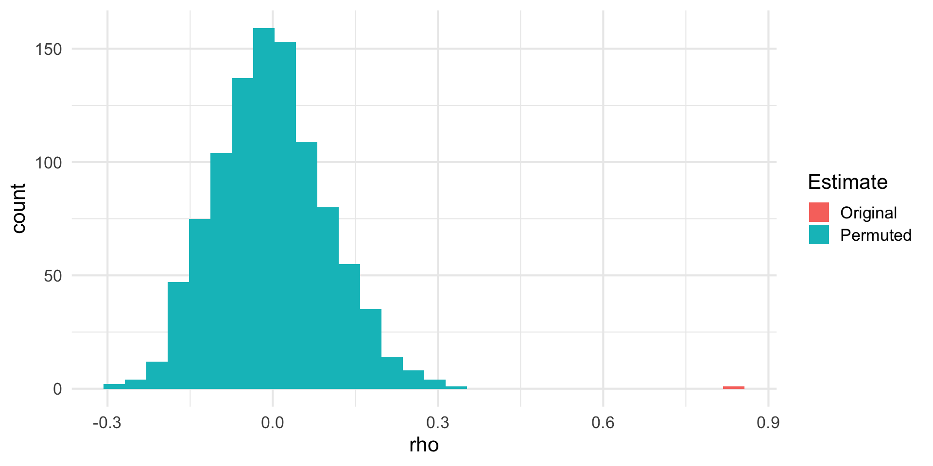
Visualizing the NULL
Probability of a value as extreme or greater than the original estimate \(\to\) P-value.